Visualizing Baltimore with R and ggplot2: Crime Data

The advent of municipal open data initiatives has been both a blessing and curse for my particular brand of data nerd. On one hand, it has opened up the possibility of developing deep and useful knowledge about the places we live and work. On the other, it opens up the possibility of starting projects to develop deep and useful knowledge about the places we live and work that inevitably get sidelined by the next deadline at work or by the basement that needs cleaning.

I collect such projects. There are about a dozen currently on a list that I have invested some amount of time in. At the current rate, I will finish about 12 by the time I die...but the list will have quadrupled.

My wife and I recently purchased a home in the Mount Vernon neighborhood of Baltimore, moving up from Washington, DC. One of Baltimore's many nicknames is "the City of Neighborhoods", and it is probably the most apt. The city is full of clusters, and arbitrary but obvious lines that separate this place from that place, and these people from those people.

The only exercise regime that I have been able to get myself to stick to over the years is running outside, no matter the weather. This is because the only way I can trick myself into keeping moving is to give myself an artificial destination somewhere X miles away or to give myself a direction to run in towards places I haven't yet been. It's a way for me to romanticize the process of making sure my stress levels stay manageable and my body doesn't slowly atrophy in front of this computer.

This habit has allowed me to cross a lot of those lines in a relatively short time here and I've tried within reason to cross some that maybe white dudes in jogging pants aren't expected to cross. No matter where you are in this city, one of those particular lines isn't far and once you cross one, you know it.

All that to say that I'm currently finishing up an intro to analytics in GIS class, and for my final project I chose one of those interests I'd collected but done very little about: using the fantastic wealth of data here to learn more about this city that I'm now calling home.

I'm building a lot of maps using good old ggplot2 for this project, and they're so pretty. There's already lots of ggplot2 mapping blog posts but in the interest of sharing that pretty, here's another.

Obviously:

## Crime Incident Plots
library(ggplot2)
library(foreign)
library(stringr)
library(lubridate)
library(plyr)
library(xtable)
library(scales)
library(RColorBrewer)
library(ggmap)

## gis libraries
library(maptools)
library(sp)
library(rgdal)
library(spatstat)

Then pulling in the data - shape files - using some of the great (but mostly HORRIBLY documented) GIS packages available in R, first the city boundary:

city_shp <- readOGR(dsn='Baltcity_20Line', layer='baltcity_line')

and I store the original map projection. I've always had a bit of a map fetish, and learning details about the different projections have been way more fun than they should be. First thing to note is, these shapefiles are not in the latitude/longitude coordinate system. If I want to convert them to lat/long, there's a function for that:

#city_shp <- spTransform(city_shp,CRS("+proj=longlat +datum=WGS84"))

But it's commented out because I don't want to do that. The projection they're currently in allows me to treat the distances between points as though they were on a plane, as opposed to a sphere. This is ok as my window of analysis is fairly small (just Bmore) and makes clustering and model fitting much more simple mathematically. It allows me to use more general tools in that part of my analysis. In fact, I'll store the original projection, and convert other data given to me in lat/long to it later on:

origProj <- city_shp@proj4string ## Store original projection

ggplot2 only takes data frames, so I gotta convert the shape files to a data frame representation:

city_pl_df <- fortify(city_shp, region='LABEL')

For all the city-wide plots, I use the city line as the first layer, so I'm going to store it as my "bound" blot and gray out the surrounding area in the plot background:

bound_plot <- ggplot(data=city_pl_df, 
aes(x=long, y=lat, group=group)) +
geom_polygon(color='gray', fill='lightblue') + 
coord_equal() + theme_nothing()

By itself, eh:

So how about all those neighborhoods then? Pull in the shape files and convert them to a data frame the same way:

## Neighborhood Shape Files read in v1
nbhds_df <- read.dbf('Neighborhood_202010/nhood_2010.dbf')
nbhds_shp <- readOGR(dsn='Neighborhood_202010', layer='nhood_2010')
origProj <- nbhds_shp@proj4string ## Store original projection
#nbhds_shp <- spTransform(nbhds_shp,CRS("+proj=longlat +datum=WGS84"))
nbhds_pl_df <- fortify(nbhds_shp, region='LABEL')

and THIS is why Baltimore is the "City of Neighborhoods":

## plot nbhd boundaries
nbhds_plot <- bound_plot + 
geom_path(data=nbhds_pl_df,color='gray')

I'm looking at lots of different datasets for this project. Some are point datasets, like 311 calls and crime incidents. Some are region or place data, like building footprints, or land use. And others are pre-summarized data by area, like demographic or economic data at the census block group or neighborhood level. Visualizing your data is important in all types of analysis, but in GIS data, it's essential. For instance, crime incidents. The crime data here locked and loaded like:

crimeData <- read.csv('OpenDataSets/BPD_Part_1_Victim_Based_Crime_Data.csv')

The data are 285,415 individual incidents reported by victims of crime, in the categories:

• AGG. ASSAULT: 31,507 incidents
• ARSON: 1,948 incidents incidents
• AUTO THEFT: 2,6954 incidents incidents
• BURGLARY: 4,5168 incidents
• COMMON ASSAULT: 54,226 incidents
• HOMICIDE: 1,342 incidents
• LARCENY: 57,247 incidents
• LARCENY FROM AUTO: 40,260 incidents
• RAPE: 1,170 incidents
• ROBBERY - CARJACKING: 1,225 incidents
• ROBBERY - COMMERCIAL: 3,592 incidents
• ROBBERY - RESIDENCE: 2,720 incidents
• ROBBERY - STREET: 15,288 incidents
• SHOOTING: 2,768 incidents

The coordinates are given as text, so:

latlng <- str_replace(str_replace(crimeData$Location.1,'\$$',''),')','')
latlng <- str_split(latlng,', ')
latlng_df <- ldply(latlng[crimeData$Location.1 != ''])
crimeData$lat <- as.numeric(latlng_df[,1])
crimeData$long <- as.numeric(latlng_df[,2])

The coordinates are given mostly (4,477 rows with no coordinates, and 6 rows in the same projection as the shapefiles) in latitude/longitude, and like I said before, distance between two points in lat/long gives distance on the surface of a sphere. so I gotta convert it:

## Convert lat/long to maryland grid
latlng_df2 <- crimeData[,c('long','lat')]
latlng_spdf <- SpatialPoints(latlng_df2, 
proj4string=CRS("+proj=longlat +datum=WGS84"))
latlng_spdf <-  spTransform(latlng_spdf,origProj)
latlng_spdf_coords <- coordinates(latlng_spdf)
crimeData$long <-  latlng_spdf_coords[,1]
crimeData$lat <-  latlng_spdf_coords[,2]

When I'm doing this kind of exploratory visualization, I like to store my plot parameters in a named list like this:

crimeCols <- brewer.pal(12,'Paired')

crimeTypes <- list('RAPE'=c(crimeCols[1],crimeCols[2]),
'ARSON'=c(crimeCols[1],crimeCols[2]),
'COMMON ASSAULT'=c(crimeCols[3],crimeCols[4]),
'AGG. ASSAULT'=c(crimeCols[3],crimeCols[4]),
'SHOOTING'=c(crimeCols[5],crimeCols[6]),
'HOMICIDE'=c(crimeCols[5],crimeCols[6]),
'ROBBERY - STREET'=c(crimeCols[7],crimeCols[8]),
'ROBBERY - CARJACKING'=c(crimeCols[7],crimeCols[8]),
'ROBBERY - RESIDENCE'=c(crimeCols[7],crimeCols[8]),
'ROBBERY - COMMERCIAL'=c(crimeCols[7],crimeCols[8]),
'BURGLARY'=c(crimeCols[9],crimeCols[10]),
'LARCENY'=c(crimeCols[9],crimeCols[10]),
'AUTO THEFT'=c(crimeCols[11],crimeCols[12]),
'LARCENY FROM AUTO'=c(crimeCols[11],crimeCols[12]))

crimeTypeNames <- names(crimeTypes)

Because that lets me loop through and plot all the subsets much more easily.

## By crime type
for (crimeType in crimeTypeNames){
## All Incidents Densities
    ttl <- str_replace_all(str_replace_all(crimeType, '\\s', '_'),'_-_','_')
    crimeDataSubset <- subset(crimeData,
    (description==crimeType))
    p <- nbhds_plot + 
    geom_point(data=crimeDataSubset,aes(group=1), 
        shape='x',
        color=crimeTypes[[crimeType]][[1]],
        alpha='.8', guide=F) +
    stat_density2d(data=crimeDataSubset,aes(group=1), 
    color = crimeTypes[[crimeType]][[2]]) +
    annotate("text", x = 1405000, y = 565000,
    label=paste(
    str_replace_all(str_replace(ttl, '_', '\n'),'_',' ')
    , sep=''), size=8) +
    ggsave(paste('img/',ttl,'.png',sep=''))
}

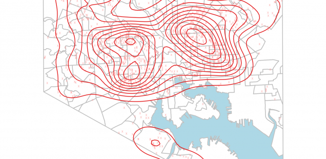
The loop above plots incidents and 2d kernel density estimates for all the crime types, allowing us to compare and contrast.

This allows us to see that while people get beat up all over the city...

...they really get shot and/or killed in mostly just East or West Baltimore.

And while people steal FROM cars downtown a lot...

...they steal the cars themselves pretty much everywhere BUT downtown.

And other, very similar city wide patterns for larceny vs burglary:

The different types of robbery: first, where the people are...

...and then where the property is...

I know, I know. Everyone plots crime data. Boring. I'll put up some of the other stuff I've been doing for this project as well. But I gotta tease it out, you know?